Lead author: Rachel Levine

Co-authors: José Alfredo Durand Cárdenas, Xie He
Dwight Macomber, Eliana Lins Morandi

The chapter details the scientific and engineering challenges associated with implementing North American Supergrid concept.

 

Overview

Many site attributes dictate terrestrial underground high voltage direct current (HVDC) cable placement, as some settings are not conducive to proper cable functioning. We mainly examined the topographical, geological, physical, and chemical components of the landscape, especially soils, in order to gain insight into the most advantageous places cables may be placed underground. We also kept ease of permitting in mind, as we visualized areas held sovereignly or have protected status. Our study reached several conclusions regarding the relative positive and negative impacts of the North American Supergrid’s  construction and operation:

• By diversifying energy sources, the NAS (NAS or the Supergrid) has the potential to save over 400 billion gallons of water per year based on current electricity demand, and may reduce the emission of several criteria pollutants.
• Should the NAS share right-of-way (ROW)space with fiber optic cables, it is imperative that HVDC cables be placed parallel to fiber optic cables. In the instance of a single existing fiber optic cable, HVDC cables should be located below and parallel to the fiber optic line.
• The magnetic field output from properly functioning cables could affect the migratory capabilities of land animals, as well as the directional orientation of compasses, to a limited extent. We do not anticipate any negative impacts on human health.
• The regulation of both heat dissipation characteristics and the relative electrical resistivity of the ambient environment are crucial to efficient HVDC cable functioning.

Additionally, we analyzed two hypothetical case studies to demonstrate potentially important siting variables in both onshore and offshore cable placement. For onshore cables, we conducted a feasibility analysis for a preliminary route for a ‘Western Pilot Project’ by analyzing several variables relating to soil composition and natural formations. For offshore cables, we mapped environmental and technical realities that may impact siting on the Atlantic Cost, allowing a determination to be made regarding the placement of onshore-offshore substations linking a potential offshore wing of the NAS to the onshore nodal network. Several environmental characteristics overlapped in their importance to both onshore and offshore cable configurations in this combined feasibility effort:

• Depth to bedrock
• The presence of protected species/land areas that house protected species
• The presence of existing oil and gas infrastructure

Overall, this feasibility analysis concluded that the positive environmental impacts of the NAS system will enable far outweighs any minimally negative externalities.

 

Introduction

Variations in the natural landscape have a clear effect on the hypothetical construction of the national grid. Soil properties are perhaps the greatest limitation that grid designers and construction teams face. Should designers use native soils to surround cable and backfill trenches, the soil must maintain critical moisture values to ensure proper heat dissipation. Similarly, natural hydraulic systems (namely water migration patterns) must be maintained despite soil changes. Variations in the depth to bedrock can also affect costs and construction time. Taking these and other similar considerations into account, this section outlines crucial feasibility considerations regarding the NAS’s environmental impacts and technical challenges.

The proposed underground HVDC grid would be best implemented by building a nodal bidirectional system. This configuration enables maximum resilience and flexibility in the bi-directional transportation of electricity with minimal environmental and mechanical interferences. Because the electric and magnetic fields originating from transmission cables are static, any negative effects on human or animal health from either field type can be considered minimal. It is possible that the NAS would have minor impacts on the migratory capabilities of flightless land mammals and/or insects in the immediate vicinity of a cable right-of-way stretch due to weak magnetic fields originating from the transmission line. Magnetic directional compasses may also become slightly disoriented from this effect. While the underground system configuration does not directly reduce the impact of such fields, cables themselves would be less susceptible to an electromagnetic pulse (EMP) attack or extreme weather event (a valuable safeguard not afforded by unshielded above-ground lines). We conclude that, while surveyors must use caution to minimize environmental impacts, the negative impacts associated with the implementation of an underground HVDC grid are insignificant compared to the benefits that it would achieve regarding national security and carbon reduction.

We begin with examining how soil properties impact cable placement, which would ultimately ensure proper functioning of underground cables in the host environment. Further, the environmental risks and benefits of implementing a nationwide HVDC system were examined, with conclusions drawn regarding the relative impact the system would have on the surrounding environment and living beings. Lastly, we examined two case studies to determine the viability of the NAS in varying environments, with promising results.

 

Siting in the Context of Soil Properties

Since the NAS will be constructed in a [mostly] underground configuration, the soil conditions of the host environment will be pertinent to proper system functioning. While surveying must be completed to confirm proper cable placement, information about a soil’s categorization (coupled with knowledge of the field of soil mechanics) can provide a strong indication of which soils should be considered suitable for underground cable placement. Soils deemed unsuitable require “amendment” before use; that is, native soils must be removed and replaced with manmade fill. The physical and chemical properties of soil will also influence its interaction with foreign materials. For the purposes of this analysis, a “physical” property will be defined as a trait that does not require manipulation of the soil’s natural state of matter to be expressed or measured;[1] physical properties include electromagnetic properties, texture, water content, and electrical and thermal resistivity (among others).[2] Additionally, “chemical” properties are those that may be evident only after or during a chemical reaction of some kind (common examples include oxidized trace metal content, salinity, pH, and natural organic matter (NOM) content).[3] The inherent soil properties displayed in various soil samples may give strong indications as to the functioning of underground cables.

 

Siting Based on Soil Orders

To identify and classify the bulk-physical and chemical properties present in soils in the contiguous United States, soils are sorted into several hierarchical categories based on their properties; there are soil Orders, Suborders, Great Groups, Subgroups, Families, and Series.[4]  As the levels progress, categorization becomes more detailed and specific, with “orders” serving as the most general classification. Globally, there are twelve soil orders: Alfisols, Andisols, Aridisols, Entisols, Gelisols, Histosols, Inceptisols, Mollisols, Oxisols, Spodosols, Ultisols, and Vertisols.[5] Each order possesses general properties that have the potential to interact negatively or positively with multiple electrical components of the underground network. Therefore, each must be carefully analyzed and assessed for risk potential. Keeping in mind the extent to which the physical and chemical properties described above will influence system functioning, the twelve United States Department of Agriculture (USDA) soil orders were determined to be either suitable (potentially without amendment) or unsuitable without amendment. Classifications should be taken as tentative until surveying is completed, as soils within a right-of-way may be disturbed or mixed, altering their properties from the ideal case.

 

Alfisol – SUITABLE

Alfisols are a clay based soil usually derived from vegetation found in forests and/or savannahs in temperate environments. They contain a modest level of organics which gives them enough agricultural potential that they could support a shorter growing season. Moisture content fluctuates strongly based on the season, allowing for the potential moisture levels to be high. Additionally, sublayers of this soil have the potential to contain oxidized iron or aluminum (that can attach to the clay itself), or other minerals such as quartz. This sublayer’s depth will dictate any resistive potential, as clay base itself has low resistivity; the more clay that is present, the lower the resistivity will be.[6]

 

Andisol – UNSUITABLE

Andisol is a very specific soil order denoted by a primary composition that is made up of volcanic ash. It has the potential to have an extremely high mineral content, yet these minerals are usually non-crystalline (which is glass based and not metallic in nature). Andisol can retain massive amounts of moisture because it is not very densely packed; its organic concentration varies based on location. Alloys (i.e. amorphous metals) can also be present in high quantities and act as excellent conductors (potentially interacting unpredictably with an HVDC system).[7]

 

Aridisol – SUITABLE

Aridisols are often found in dry desert regions, and can best be described as sand-based with poor moisture content and little to no organics. Sublayers usually contain silica, salt, gypsum, or calcium carbonates (all of which are generally poor conductors when compared to metals). Potentially high temperatures, coupled with the potential for very little moisture recharge, are concerns when the prospect of a thermal runaway is considered. Built-in protections against this phenomenon around the HVDC cable itself must be evaluated further to utilize this soil order without amendment.[8]

 

Entisol – SUITABLE

Entisols are relatively under-developed soils that lack fully formed horizontal layers. Formations of this order are usually due to some form of disturbance, such as erosion, and are further formed by either a very dry or very wet environment. This soil type is predominantly clay and sand, yet has no clear or predictable composition. Furthermore, a variety of materials can contribute to formation including dense rock, highly compacted soils, or even toxic waste. Moisture content can also vary widely, compounding resistivity issues already present due to the formation material. Locations must be surveyed carefully before non-amendment use if they contain Entisol soil.[9]

 

Gelisol – UNSUITABLE

Gelisols contain glaciated deposits which are characterized by thick impenetrable permafrost layers (such as those found in tundra environments). They are well-known stores of organics, yet are only formed in very cold environments and therefore, do not support the growth of most plants. This frost layer introduces resistivity concerns. Additionally, the permafrost layer will most certainly hamper or halt trenching efforts and therefore should not be considered usable ground without extreme amendment.[10]

 

Histosol – UNSUITABLE

Histosols are primarily composed of organics and are commonly found in peat rich bogs or swamp environments. The organics in the soil have a strong potential to oxidize other soil constituents, allowing for decomposition to occur rapidly due to the anaerobic conditions present when soil is completely immersed in liquid. Logistical construction problems could arise due to the potential for the soil’s texture to be inconsistent. Having a high concentration of organics, that act as heat insulation material, these soils should not be considered suitable for cable undergrounding without amendment.[11]

 

Inceptisol – SUITABLE

Inceptisols form in a multitude of environments (like Entisol soils). Ultimately, Inceptisols typically contain a larger than usual quantity of organics and moderate moisture retention ability. Minimal accumulation of oxidized metals, clay, and organics can occur, but rarely in the amounts that would exceed present detection limits. This order is usually present within mountainous areas, but contains low erosion potential. Ultimate usage is dependent on the depth bedrock level in these mountainous areas.[12]

 

Mollisol – SUITABLE

Mollisols are characterized by a layer of grassy vegetation followed by a layer of dark organically rich humus soil. They often have high moisture levels, leading to saturation during some seasons. However, the lack of toxic or troublesome compounds mitigates this concern. Mollisols must be surveyed before use without amendment to determine the depth of the organically rich layer directly below the topsoil.[13]

 

Oxisol – UNSUITABLE

Oxisols are characterized by their low nutrient/organic levels, low concentration of electrolytes, and high concentrations of oxidized metals. This is due to the fact that oxisols are usually located in humid environments with very acidic pH levels, which leads to favorable oxidation conditions. They usually contain moisture but do not readily retain it. The extreme acidity of these environments could prove to be unfavorable for the outer sheath of the HVDC cable.[14]

 

Spodosol – UNSUITABLE

Spodosol soils contain three distinct layers; a rich organic surface topsoil, an ash-based sublayer, and a reddish horizon layer (due to high iron content). Generally, subsoils in this order have both a low organic content and a low clay content. Organics in the top layer have a strong potential to oxidize metals within the soil, which can flow down into the sublayers since the base soil usually has a sandy texture with favorable permeability characteristics. Moisture content can vary, but tends to be high when rainfall exceeds evapotranspiration removal rates. The relatively uninhibited transference of problematic materials throughout the layers could pose issues for grounding equipment present along the length of the HVDC cable. Therefore, Spodosols should be amended before hosting cables.[15]

 

Ultisol – SUITABLE

Ultisols are mineral rich clay based soils (which sometimes contain oxidized iron, namely due to the low pH conditions) and quartz. The moisture content of Ultisols varies widely depending on where they are formed. Nevertheless, soil fertility is low due to a lack of organics and electrolytes, which leads to a texture that promotes mineral leaching throughout the soil horizons. Surface soils tend to be more hospitable, yet can still contain these troublesome minerals. Due to the shallow depth of cable trenches, it is reasonable to assume that the cables will most likely be laid in this more hospitable area.[16]

 

Vertisol – UNSUITABLE

Vertisols are clay based soils, rich in calcium, magnesium, and lime, that respond dramatically to changes in water content by shrinking and swelling. Such activity can cause deep cracks within the soil layers during times of low moisture. In high moisture periods, water tends to settle in the topsoil of this order, and can even collect standing water. This unpredictability will not only be troublesome during the construction period, but also could cause issues with the thermal regulation of cables (particularly regarding heat dissipation), and should be avoided without extreme amendment.[17]

Should soils contain favorable properties as described above, it would be possible to bury cables in native soils directly, thus eliminating the use of cable sand entirely in certain line stretches (as long as no large boulders or stones are present). The possibility of utilizing native soils as fill materials must be evaluated on a case-by-case basis once cable routes are established, usually by means of surveying and moisture testing. The properties of native soils in such areas (described by soil orders) could possibly be used as a guide to pinpoint optimal sampling locations during the initial construction phase of the NAS.

If native soils are unsuitable, amendment by way of “backfilling” may be employed as a cost effective and simple construction technique, during which existing soils are replaced with artificial fills before in-ground cables are placed. The area immediately surrounding the cable and its electrode may require an engineered soil fill to both regulate and stabilize the thermal properties (even when the material itself is dry),[18] a crucial component to the proper function of HVDC cables. Engineered soil parent material can vary based on the geographical source of the materials relative to the construction site. However, modern engineered fills, such as Fluidized Thermal Backfill, typically include sand, cement, and aggregated minerals.[19] When compared to native soils, engineered soils not only consistently achieve proper moisture levels, but also allow for proper compaction (without the possibility of soil contamination during the process).[20] Trenches housing cables are often refilled with a maximum of 50% existing soil as an economical technique to prevent lasting ecological disturbance.[21]

It is also vital to note that not all existing engineered soils can be utilized in an HVDC system. For instance, typical highway construction methods require the presence of several engineered layers that are not conducive to grid construction. These are the two layers that are usually present underneath a paved road, the “base course” and the “subbase.”[22] While the thickness of these layers is dependent on the quality of the native soil, both of these layers typically contain aggregates of high resistivity, such as granite, and are heavily compacted to form a single layer.[23]˒[24] However, the use of highway right-of-way could still take place next to a paved surface in native soil, or along the highway median.[25] This presents a considerable advantage, considering all locations containing major highways are typically tested for soil quality before construction, much like an HVDC grid. In contrast to the highway support materials, a railroad subgrade is not as densely packed at the surface. This is due to the “ballasts” that are made up of loose stones, which are compacted (and not cemented in place) to form a single layer on rail tracks.[26] If necessary, it could be easier to possibly insert HVDC lines directly underneath railway lines in the natural soils below, (depending on their overall depth). This alternative must be explored further by installation contractors throughout the initial surveying process.

 

Siting Based on Soil Resistivity Trends

Soil science is influenced by two distinct types of resistivity: thermal resistivity and electrical resistivity. Thermal resistance is the ability of a material to resist heat dissipation (or, the movement of heat away from a source),[27] whereas electrical resistance is a measure of a sample’s potential electrical conductivity.[28] Furthermore, there is no direct mathematical method to compare one value to another in the realm of soil science (this can be done only if one is interested in comparing electrical and thermal resistance in metals).[29] Electrical resistivity is expressed in terms of  (Ohm- meter) whereas thermal resistivity is expressed as  (Kelvin-meter/Watt, where “Kelvin” is a unit of temperature). Therefore, electrical and thermal resistivity will need to be analyzed separately for the same area of soil using different techniques. Despite this fact, there is a direct and simple relationship between resistivity and conductivity that can be applied to both electrical and thermal calculations. Conductivity can be expressed as the inverse of resistivity, and vice versa. This implies that one value can be transformed into the reciprocal to get its corresponding resistivity or conductivity quantity. While an exclusive study of soil properties (without field surveying thereafter) is, at best, a tentative approximation for resistivity, such an analysis is nevertheless a promising guide as formal surveying begins.

Both resistance phenomena will separately affect a HVDC grid, with an increase in either thermal or electrical resistivity resulting in similar negative results for both the cable’s current rating (i.e. the ability of the electricity to flow through the cable while staying within optimal temperature limits, based on manufacturer specifications) and its subsequent wattage. If thermal resistivity is high, heat becomes trapped close to the cable’s surface. As the cable’s temperature increases, its electrical resistance also increases, resulting in higher power losses (denoted by the formula: I²R); these losses then further increase the temperature, causing a cyclic trend referred to as “thermal runaway.” If the thermal resistance value is unfavorable, the current may still flow, but the actual current rating may decrease to prevent cable overheating. In more extreme cases of a very high thermal resistance value, the same trend will initially occur, but eventually the process of heat production, entrapment, and increasing power losses will cause the entire system to overheat and collapse.

Thermal and electrical resistivity are strongly influenced by three indicators: salt content, moisture levels, and temperature. These indicators are often dictated by soil composition and the concentration of chemical constituents, if present. Thermal probing of field sites is often required to properly determine if the host soil contains favorable moisture properties. This information is necessary to determine how soil moisture relates to its relative thermal resistivity value, a relationship depicted in a “soil thermal dry-out” curve. If the critical moisture value is not met or exceeded, the lack of moisture will be further exacerbated by way of cable heat, driving away what little moisture that is present.[30] A lack of heat transfer between the HVDC cable and its surroundings can cause a dramatic increase in the temperature of the cable itself, ultimately causing thermal runaway. The soil thermal dry-out curve can also yield clues as to the behavior of a system during times of surplus moisture. The asymptotic behavior of the curve signifies that the critical moisture point has been reached and exceeded. Thereafter, the thermal resistivity will most likely not reach zero, but simply trail along the asymptote as moisture continues to increase. This implies that excessive moisture does not cause any additional significant reduction in thermal resistivity after the critical moisture point is reached. When this information is coupled with the possible negative consequences of excess moisture outlined below, it is reasonable to conclude that excess moisture situations must be avoided, as they add no positive attributes to the system. Field testing should be completed to gather data for an accurate dry-out curve representation prior to grid installation.

As moisture content increases, a soil sample’s thermal conductivity value tends to increase because air has a significantly lower thermal conductivity rating when compared to water. Water aids in increasing contact between the individual soil particles, allowing for heat to easily flow away from the source.[31] Electrical resistivity of the soil tends to decrease with higher moisture values as chemical constituents, such as electrolytes, become activated around conductors. For the purposes of HVDC application, the moisture content of the cable’s direct surroundings should be a minimum of 10%, as resistivity increases significantly when moisture content falls below this level.[32] Similarly, it is generally accepted that electrical resistivity is high when the moisture content of soil falls below 10%.[33] Indeed, field-derived sensitivity tests focusing on the relationship between soil salinity and moisture, conducted by AEMC Instruments, were not even conducted at conditions below 15% moisture.[34] While moisture is clearly a critical component of suitable soils, it must be noted that excessive moisture can also cause two kinds of problems. First, moisture can cause corrosion over time due to its potential to interact with other soil constituents around the cable,[35] stimulating chemical reactions. Second, waterlogged soils are more likely to cause the formation of a frost layer, which can dramatically increase both types of resistance, even if the host soil order is favorable during warmer seasons.[36]

Typically, soils that are low in moisture and electrolyte (free ion) concentrations introduce the most electrical resistance; solid stone and volcanically derived soils are prime examples of this phenomenon.[37] The depth to bedrock (discussed subsequently in the section entitled “Siting in the Context of Geology, Topography, and Contamination”) and presence of solid rock fragments present within the immediate area must be accounted for during surveying to accommodate this trend. Generally, electrical resistivity decreases as salt content in soil increases.[38] This is because sodium chloride (along with many other salts) is a strong electrolyte,[39] meaning that it will completely ionize in water by breaking into the charged elemental components of its molecular structure. These ions then become mobile in solution and improve conductivity by shuttling electrons.[40] It should be noted that ionization does not imply dissolution. Every particle does not have to break into its positive and negative elemental components for improved conductivity to occur. Being a “strong electrolyte” simply implies that when the molecular compound does break down, it completely ionizes.[41] Ionization must first occur for salts to lower levels of electrical resistance. Therefore, the moisture content is an intertwined soil component that is often measured concurrently with salinity.

When wet, naturally occurring sand deposits possess high relative thermal conductivity compared to conventionally favorable soils, such as clay.[42] Soils rich in clay and sand tend to possess higher thermal conductivity values compared to soils rich in NOM, which tends to insulate cables and prevent heat transfer to the ambient environment.[43] Salt content is usually measured as its percent weight in moisture, as the ability of a soil to retain moisture will often drive its concentration of electrolytes. Well-graded soils, with multiple granular sizes, or porous sandy soils that are notorious for low moisture values should similarly be expected to have low naturally occurring electrolyte values, even if salts are present. Even if soils do not have naturally occurring salts, electrical resistivity may still be low if enough moisture is present. As shown in an analysis of electrical resistivity in terms of moisture content, AEMC Instruments found that moisture contents below 20% were much more susceptible to disproportionally large increases in resistivity, compared to more saturated soils found at a constant above-freezing temperature.[44]

Temperature, the final indicator of thermal and electrical resistivity, is influenced by both moisture levels and salinity. Generally, soils with very low temperatures tend to have high electrical resistivity values, especially at temperatures which allow the moisture present within soils to freeze. Similarly, soils with higher levels of moisture tend to lower, or maintain lower, temperatures over time.[45] An important deterrent to the obstacle of soil moisture freezing is the presence of salts (which may possess varied elemental make-ups in nature). While salts do not totally prevent increases in electrical resistivity associated with temperature drops, they tend to lessen the severity of these fluctuations. Ultimately, soil temperatures appear to be the overarching condition which determines soil fitness in both quantitative and qualitative approaches. Not only does temperature influence moisture levels, and vice versa, but it can also heighten, or lessen, the impact of soil thermal resistivity on current ratings. Most common soil types tend to require 15% – 30% moisture content in temperate environments to maximize cable functioning, according to our own calculations.

 

Siting in the Context of Geology, Topography, and Contamination

The natural surface characteristics of the earth can greatly influence construction of the NAS. Geological bedrock formations, as well as surface characteristics, which can be both natural and anthropogenic, have the greatest potential to slow down or halt construction. To construct the NAS efficiently, as much preliminary siting as possible should be completed to prove project feasibility in conditions where land restrictions and non-project related manmade infrastructure are present. This section surveys how landscapes, geology, and manmade environmental interferences impact soil siting.

 HVDC cables should be laid at a minimum depth of 1.2 meters below the topsoil whenever possible. This 1.2 meter depth is both deep enough to maximize protection against accidental tampering, while allowing for ease of access during cable maintenance. When deciding where to lay cable, it is especially important to note the presence of shallow bedrock layers, as the process of cutting through such a layer is time consuming, costly, and potentially environmentally hazardous. Bedrock is often removed by blasting, which “fractures” the formation, and can potentially cause temporary groundwater contamination.[46] We used high-resolution nationwide data banks to visualize areas which require further investigation due to the complexity of bedrock formations. Since the NAS will ideally be built upon existing rights-of-way, such geologic features will be crucial to identify, and avoid if possible, near highways and rail lines.

Foreign objects, either natural or artificial, can complicate underground cable placement. To ensure cables consistently function properly, they must not encounter any foreign objects in soil, and several measures must be taken to prevent such interaction. First, the removal of trees directly on top of and immediately near a given right-of-way stretch is essential. This ensures that roots do not become entangled in cable trenches or around cables. We do not anticipate that tree removal will be a large factor during cable installation, as this process has likely already been completed along highway medians or in highly developed areas. In virgin (or, previously undeveloped) lands, tree removal must be conducted with caution to ensure that the local biosphere traits are maintained. Ultimately, the usage of virgin lands should be avoided when possible. If left in place, nearby trees or larger plant developments must be monitored to ensure that no roots encroach on the HVDC trench over time. Manmade infrastructure in the form of oil/gas transportation pipelines must also be circumvented. Should a HVDC line failure occur, free electricity will often jump to and charge metallic objects nearby, including oil and gas infrastructure; this in turn may create dangerous conditions that could damage both the conductor itself and any other manmade infrastructure nearby. To avoid this, we mapped oil and gas infrastructure in the continental United States and compared these routes to proposed cable routes. HVDC cables may also compete for underground space with fiber optic cables, which are often used in the telecommunications industry. (We discuss the possibility of co-placement and/or usage of fiber optic cables in the NAS system below in the subsection entitled “Potential System Interferences”).

In addition to the presence of possible physical obstructions to HVDC cable placement, some land areas may be restricted due to government regulations or miscellaneous soil-related environmental hazards. Throughout the contiguous United States, the designation of a certain land area as a “protected area” restricts development in National Parks, biodiversity conservation areas, and some federally owned lands (such as military bases). While dozens of “protected” designations were analyzed to ensure that the NAS avoids passage through such areas, the most critical restrictions placed on siting for the new grid were the avoidance of GAP (National Gap Analysis Program) 1 and 2 status lands. GAP Status 1 is defined as “an area having permanent protection from conversion of natural land cover and a mandated management plan in operation to maintain a natural state within which disturbance events (of natural type, frequency, intensity, and legacy) [can] proceed without interference or are mimicked through management”.[47] These are areas with strict rules against construction of any kind to protect biodiversity and/or endangered species. In GAP Status 4 areas there are “no known public/private institutional mandates/legally recognized easements.”[48] Areas with GAP Status 3 can be subject to extraction uses, such as mining and logging. Data pertaining to the presence of Native American sovereign lands was also collected from public sources.[49] While this analysis allowed for the potential placement of cables in sovereign areas, future collaboration must occur if the final cable route passes through these lands to ensure that the opinions of tribal leaders are considered, particularly regarding sacred areas (which should not be infringed upon).

Lastly, hazardous environmental disturbances must be accounted for and avoided during cable placement to ensure proper cable functioning and, more importantly, to protect the outer protective casing of the cables themselves. We have mapped out land areas of known contamination, namely Superfund and Brownfield locations, that should be avoided as route siting continues. Similarly, we eliminated conditions which could cause the corrosion of concrete conduits surrounding the cables. Such corrosive conditions can stem from either anthropogenic interference or natural causes. Concrete corrosion potential was rated to indicate “low”, “medium”, or “high” risk by considering variables such as soil acidity.

 

Environmental Risks and Benefits

The North American Supergrid will enable the avoidance of the majority of power sector carbon dioxide emissions if implemented as outlined by the foundational MacDonald et al. publication (described previously). However, the scale of the NAS means that numerous geographical regions will be impacted by its construction. So far, few immediate environmental or health risks stemming from NAS implementation have been identified, given that proper installation procedures are used and extensive environmental impact assessments are completed. This section presents what we know about these risks at present. It should be noted that this technical analysis is the most representative of any possible effects of the development of virgin land. Presumably, burying cables along existing transportation avenues would not drastically change the ecologically disruptive tendencies of existing infrastructure.

 

Avoidance of Terrestrial Ecological Risks

The magnetic field output from cable operation could affect the migratory capabilities of land animals to a limited extent. Animals in contact with ground surfaces and residing up to 1.5 meters above the surface will most likely be the most susceptible to field output along the length of any overhead or underground direct current (DC) line (likewise for compasses used at such locations). The presence of highways has most likely already caused some form of ecological disturbance in the area, especially if the land surrounding the roadway has already been developed.[50] In the very rare case that virgin lands, or remote railway rights-of-way, must be used to accommodate cables, the ecological impacts of magnetic field contact at the specific setting should be evaluated and resolved if possible. In any area of high animal activity, fencing or other physical deterrents may be used to further prevent ecological risks and structural damage.

 

Avoidance of Marine Ecological Risks

The prospect of placing cables in marine environments presents unique environmental challenges. Cables must be able to withstand extreme pressure and saline conditions, while the surrounding environment must be able to rebound and thrive after cable installation is complete. In this section, we discuss two crucial considerations linked with marine cable placement, chlorine gas emission and magnetic field interference. The section entitled “Case Study 2 – Atlantic Coast Submarine Project”, paints a more detailed picture of chemo-physical, biodiversity, and anthropogenic siting considerations along the Atlantic Coast of the United States.

Chlorine gas is produced in HVDC submarine cables at the anode of a monopolar system, where the electrical current interacts with the surrounding water through the process of electrolysis.[51] During ocean electrolysis, salt dissolves into positively charged sodium ions and negatively charged chloride ions. These ions then combine with the electrons originating from the anode to form gaseous chlorine.[52] While chlorine gas is highly toxic and corrosive, especially in aqueous environments,[53] it can only be produced in a monopolar HVDC configuration. The literature has noted that the use of bipolar systems, as is proposed for usage in the NAS system, virtually eliminates the risk of chlorine gas production in underwater HVDC systems.[54]

There is concern about the potential disorientation of aquatic organisms that rely on Earth’s magnetic field to migrate near HVDC cables. This issue of magnetic interference originating from underwater cables has been studied extensively. Yet, the literature has not reached a consensus as to the effects on migrating marine life, in part due to the mystery surrounding the mechanism whereby various land and aquatic organisms orient themselves.[55] During the installation of the SwePol HVDC link, an underwater monopolar HVDC link between Sweden and Poland, researchers concluded that the usage of a bipolar configuration significantly lowers magnetic field interference when compared to monopolar systems due to the partial cancelling of fields in opposing directions.[56] Furthermore, shallow buried cables often only emit a strong magnetic field directly above the cable location, with some systems indicating a significant drop in magnetic field distortion at a horizontal distance greater than 5 meters from the cable.[57]

While these considerations suggest that cables are generally safe for the surrounding oceanic environment, it is still prudent to take basic safeguards to further protect aquatic species. Cables should be buried in the deepest seabed possible, preferably in the oceans’ dysphotic zone (at least 200 meters below the water surface). In this zone, photosynthesis cannot occur and sunlight diminishes rapidly as depth increases.[58] This may minimize the risk posed to many endangered species and commonly consumed fish, which usually reside closer to the surface. In addition, any protected coral reef formations must be mapped beforehand and carefully avoided during the installation process. Although marine environments have been proven to successfully rebound after disturbances by cables, the fragility of many reef ecosystems makes such resilience an unlikely trait.[59] Analysis of potential species interactions and any disturbances to fishery activities must be accounted for during the installation and operation submarine HVDC cables.

 

Possible Public Health Concerns

To date, the majority of studies attempting to quantify the health impacts of HVDC lines have been conducted using above-ground configurations. Even so, we can learn quite a bit about the potential of underground HVDC lines to interact with humans, animals, and inanimate objects in their immediate surroundings from these studies. Ultimately, the literature suggests that magnetic fields associated with HVDC outputs do not have the potential to impact cell growth or reproduction capabilities.[60] Impacts on the migratory abilities of land-bound animals positioned very close to cable beds are the main health-based consequence of HVDC line operation.

Magnetic fields produced by HVDC line operation may have the potential to affect biological migration systems. As such, it is crucial to put into context the magnetic field strength associated with overhead and, by extension, underground cables. Magnetic fields of 2000 microteslas (μT) are required to impact the health of nearby animals or humans.[61] Comparatively, the magnetic field of Earth is less than 100μT at the surface. To explore the possibility of exceeding this value, we calculated the magnitude of the B-field resulting from the superposition of the magnetic fields for the two conductors when they were carrying 3000 amps in opposing directions to determine its relative strength compared to Earth’s magnetic field. If final magnetic field strength was determined to be equal to or less than that of Earth, negative health impacts were assumed minimal or negligible. The graphical representation (Figure 1) illustrates the increasing weakness of the field as it moves outwards and away from the source (3GW bipolar HVDC cable pairing with 3000 amps flowing in each direction on a single circuit), resulting in a magnetic field of negligible strength at 10 meters away from the cables on either side. The dashed line on Figure 1 represents the residual B-field of Earth, which was maintained at 40μT. It is clear that a HVDC line of significant capacity will produce a magnetic field much stronger than that of the ambient surroundings directly above and near the cable pair.

Figure 1 Magnetic field for cable pair spaced 0.3 meters apart at a depth of 1.5 meters

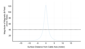
As noted above, the strength of a given magnetic field must be at least twenty times Earth’s magnetic field to impose negative health effects on humans and animals. While Figure 1 proves that this value is not broached for a 3GW line, the field produced could impact the directional capabilities of nearby mammals who utilize Earth’s magnetic field to orient themselves in their environment. However, two factors limited our ability to draw more specific conclusions about the impacts artificial magnetic fields have on migratory mammals. First, the variance between magnetic field responses of different species makes it impossible to apply a single conclusion to all affected animals. Second, in many cases, the literature lacks a firm consensus as to the mechanism that controls magnetic field responses in animals, thus making it unclear how this phenomenon even emerges. For these reasons, it should be assumed that animals in very close horizontal proximity to a buried HVDC cable and known to utilize the Earth’s magnetic field will most likely be affected by the HVDC system. This conclusion highlights the importance of utilizing existing rights-of-way whenever possible. By placing cables in previously developed land, fewer land-bound species may be impacted when compared to the same placement on virgin land.

The electrostatic fields created by above ground HVDC transmission lines have been known to produce air ions via conductor operation, in the form of charged particles.[62] There is very little research on such particles in relation to human health. Therefore, there is no set limit for maximum recommended air ion exposure for humans or animals. Similarly, several studies involving air ion output from above ground HVDC transmission lines determined that there were no conclusive changes in blood pressure, pulse, respiratory function, and body temperature due to air ion exposure. Indeed, typical car exhaust emits more air ions than an HVDC transmission line.[63] The electrostatic field, although present, also does not have the capability to “penetrate an organism,” and therefore should not be considered a harmful component of this system.[64]

Generally, the electric and magnetic fields emitted by properly functioning underground cables pose a minimal risk to surrounding lifeforms. While the migration mechanisms of many species are still not well understood, limited interference with this capability by HVDC cables is the main concern found by our analysis.

 

Potential System Interferences

As we have already indicated, electric fields do not produce major mechanical interferences in other systems. When HVDC lines are operated properly, both the resulting electric and magnetic fields remain static in nature,[65] meaning that they are constant with changes in time.[66] In such cases, the harmonic energy content and electric radio-frequency interference (RFI) that is shot into the HVDC side of station converters may radiate and impair nearby radio and telephone communications. However, grounding the metallic screens of the buried cables greatly suppresses this interference. The capacitance between the center conductor and the metallic screen wrapping serves to filter and suppress much of this high-frequency energy. Grounding the screen shields shunts these time-varying electric fields to ground.^[67] The grounding of the outer metallic screen of buried HVDC cables also serves to significantly suppress the radial voltage field of the high-voltage current-carrying center conductor. With the outer metallic screen held very near ground potential, the entire voltage drop, or rise in some situations, between the operating voltage of each cable and the local ground is constrained to occur within the insulating layer within the cable. Therefore, no significant external DC voltage fields exist.

There is, however, some risk that HVDC-produced magnetic fields could interact with unrelated man-made systems. Aside from reduced physical vulnerabilities of the network hardware, the proximity of two buried cables results in a significant reduction in the net magnetic field at moderate distances from the pair. The opposing currents in the two conductors produce opposing magnetic fields. This in turn could combine additively in the ground area between and above the cables, but oppose each other to partially cancel out either side of the burial trench. At a distance ten times the inter-cable spacing on either side of the trench, the static magnetic field is reduced to less than one-eleventh of that of a single cable.

Careful configuration of HVDC cables within highly utilized rights-of-way is essential to proper system functioning, particularly regarding the potential interactions between telecommunications and electric cables alike. Most often, HVDC technology competes for right-of-way space with existing fiber optic telecommunication cables. Fiber optic cables are a common type of telecommunication cable, and are designed for long distance, high performance data transmission. Additionally, the proper usage of fiber optic technology to transmit valuable operational information is essential to the application of software to deter cyberattacks. The center of each glass strand is called the core, which is surrounded by a layer of glass called cladding. The external optical fiber jacket and buffer tubes protect glass optical fiber from environmental conditions that can affect the fiber’s performance and long-term durability.

In shared rights-of-way, the potential for DC links to generate a magnetic field which interacts with charged particles or objects nearby (such as a fiber optic cable) is great. Depending on the magnetic field strength generated by power transmission cables and the outer electric field, the refractive index of the optical fiber material may change. This process, known as the Kerr Effect, occurs when the intensity of the light beam in the optical fiber affects the refractive index,[68] ultimately limiting high-speed (more than 10Gbps) data transmission. The Faraday effect is another phenomenon that relates the light propagated through the optical fiber and the field generated by the HVDC cables, potentially producing errors in data transmission.

The closer HVDC transmission cables are to existing fiber optic structures, the larger the electromagnetic effect over the fiber is. Therefore, determination of correct configuration for both types of cables (within a given right-of-way) is essential. NAS HVDC transmission cables should be buried at a minimum depth of 1.2 meters. Each bipolar pair is based on two parallel cables with their centers separated by a distance of 0.30 meters. Buried fiber optic cables must be located in a neutral area, far enough away from the electromagnetic source to be unaffected by it. Additionally, fiber optic cables should not cross transmission cables, since the magnetic field generated would be parallel to the propagation of light in the fiber.[1] In the case that two optical fibers were located above the HVDC cables, the value of the magnetic field would be much higher than the Earth’s magnetic field. Therefore, a fiber optic cable should be parallel to HVDC cables. In the instance of a single fiber optic cable, it should be located above and parallel HVDC cables, according to the following design:

Figure 2 Design configuration for the HVDC transmission cables and the fiber optic cable

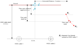
In the scenario in Figure 2, transmission cables and the optical cable must have a 0.3 to 0.61 meter soil separation,[69] implying that the fiber optic cable depth must extend from 0.61 meters to 0.91 meters. After various simulations, and considering the fact that the fiber optic cable cannot be close to the soil surface, we determined that the horizontal distance of the fiber optic cable from the center of the HVDC transmission cable should be at least 1.5 meters (at a burial depth of 0.64 meters for the fiber optic cable). In this configuration, the magnetic field generated around the fiber optic cable is approximately 17 , a lower value than Earth’s magnetic field. Additionally, to avoid coupling effects between groups of bipolar 2-GW transmission lines, a minimum horizontal distance between groupings is essential for proper configuration. Results showed that a distance of 2 meters between bipolar HVDC pairs is needed to get a magnetic field of 31  a value comparable to the Earth’s magnetic field. By applying these configuration suggestions, the NAS system can potentially work with existing infrastructure in a fortified configuration to protect against both manmade and natural disturbances.

 

Water Quality Impacts and Usage Modelling

The presence of groundwater and aquifer stores must be accounted for when designing and constructing an underground HVDC system. Not only does the construction of such a system have potential negative consequences for groundwater quality, such as temporary turbidity; it could also permanently alter water flow through natural systems. The cable sand surrounding HVDC cables and the heat the cables produce are the system components most likely to cause problems, since they have the greatest potential to interact with aquifers and subsequent groundwater stores.

The contiguous 48 states are home to thousands of freshwater aquifers of varying degrees of drinkability. The geological and topographical characteristics of a location determine the thickness of an aquifer, the depth to the water table, and the ease of access to the water supply. The distinction between confined and unconfined aquifers complicates the collection of data regarding groundwater depth and flow patterns. The depth to groundwater must be considered when building an HVDC system, as shallow, unconfined water reserves may be unnecessarily disturbed by cable trenches. An analysis not incorporating these factors could possibly cause standing water and/or well contamination. It is accordingly vital that we distinguish between the components of a groundwater system to accurately describe mapped data. The various components of a given water system are illustrated in Figure 3.

Figure 3 Groundwater formation cross-section

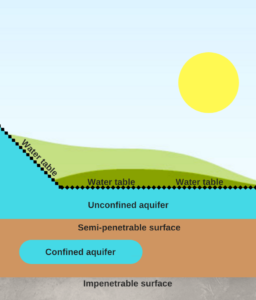
A system’s “water table” designates the top of an aquifer (otherwise known as “depth-to-water”). Its depth is relative to the corresponding topsoil layer and can change based on variations in topography, even within a relatively small area. An aquifer is deemed unconfined if there is no presence of a bedrock/impenetrable layer above the water table. In such a case, a permeable soil layer is the aquifer’s only protection from its surrounding environment. To determine the characteristics of major aquifers in the United States, the United States Geological Survey (USGS) has classified several major aquifer systems as “principal aquifers,” which are considered extensive sources of drinkable freshwater. However, wide variation in depth-to-water values in groundwater monitoring wells in such aquifers (provided through the national Advisory Committee on Water Information, a USGS subsidiary) implies that generalized conclusions regarding aquifer water table depth may be too simplistic. Therefore, NAS research has focused on visualizing all nationally available monitoring well data to inform later system refinement.

It is possible for the depth of the water table and the type of aquifer formation to impact the properties of the native soil, which in turn can affect cable function. Soils present above the groundwater table are more resistant to current flow and exhibit higher water evaporation rates,[70] because soils are typically dryer there. This exacerbates the importance of the critical water level in the surface layers of native soil. While cable or thermal sands may not directly interact with groundwater formations, they can greatly influence the groundwater flow. This is particularly important when right-of-way routes are present near highly graded, or sloped, land. In these specific cases, “trench plugs” placed at the bottom of slopes can alleviate the possibility of water flow through cable sands preferentially causing disturbance of natural groundwater movement.[71] In such high-risk areas, the possibility of eliminating the usage of cable sand entirely, if native soil is favorable, is the cheapest and arguably most effective protection against plausible hydraulic disturbances.

Furthermore, changes associated with water usage due to NAS implementation must also be estimated. Water demands from the power sector, mostly due to power generation methods, heighten competition for freshwater resources and thereby increase prices for various sectors of the economy. Changes to both withdrawal and consumption influence the stock of freshwater available. All freshwater resources removed from a water source are known as “withdrawal,” while “consumed” water is the total volume of water not returned to the original source after electricity has been generated. Consumed water is not available for future withdrawal. Comparatively, producing energy with fossil fuel or nuclear material withdraws and consumes more water per megawatt-hour than equivalent renewable generation. Therefore, most of the water savings achieved by the NAS are the result of increased renewable penetration in the electric grid.

We constructed a model to gain insight into the changes in national water consumption and withdrawal patterns due to NAS implementation. This required us to analyze current contributions to electricity generation by heavily utilized sources (such as coal, natural gas, wind, and solar), estimate likely future contributions by these sources in 2030, and calculate consumption and withdrawal values for all generators to utilize many different figures and achieve a weighted average. We concluded that, if electricity demand remains constant, the NAS has the potential to produce consumptive water savings of over 405 billion gallons yearly and withdrawal savings totaling over 14 trillion gallons yearly (if electricity demand in 2030 is equal to that of present day); these reductions equate to a 65% reduction in total freshwater usage, both withdrawn and consumed. Even if electricity demand doubles by 2030, the NAS can still potentially ensure sizable water savings compared to current usage levels.

 

Air Pollution Impacts and Emissions Modelling

Air pollutants such as ozone and nitrogen oxides will undoubtedly be released into the atmosphere during the construction of HVDC transmission systems. The resulting pollution pales in comparison to the enormous reductions in atmospheric carbon and criteria pollutants that will result from the increased penetration of renewables the NAS makes possible.

Ozone pollution from the NAS is not a significant concern. In terrestrial HVDC transmission systems, most research concerning ozone output has been conducted using data from above ground configurations. Nevertheless, the results of this research still yield important clues about the behavior of underground systems. In all HVDC systems, ozone is generated from the system conductors along the transmission line, which can produce ozone and its precursors, such as nitrogen oxides.[72] This phenomenon, referred to as the Corona Effect, influences how the transmission system interacts with its surrounding environment at many interfaces. Both the Corona Effect and subsequent pollutant discharge is dependent mainly on the environmental conditions the cable is exposed to. Hence, contact with moisture through precipitation or fog is a driving factor to determine the strength of the Corona Effect in overhead HVDC lines.[73] Scientific literature has proven that ozone concentrations specifically derived from overhead HVDC transmissions lines, with total voltages comparable to those proposed for the NAS, are consistently below detection levels during times of favorable weather when compared to ambient ozone concentrations.[74] Heavy precipitation events, which are assumed to be the worst case scenario for producing ozone emissions due to a subsequent inflammation of the Corona Effect only produced ozone cloud concentrations totaling 0.01 ppm.[75] Comparatively, 0.07 ppm is the maximum allowable daily limit of ozone exposure set by the United States National Ambient Air Quality Standards (NAAQS).[76] In American megacities, such as Los Angeles, ozone levels are frequently recorded at 0.15 – 0.5 ppm levels,[77] double the NAAQS value and a maximum of 50 times higher than ozone levels produced by HVDC technology.

We determined that implementing the NAS would have positive effects through modelling of EPA-sanctioned Criteria air pollutants associated with current and expected electricity mixes. We chose criteria pollutants as an air quality indicator due to their widely-accepted impact on human and environmental health. Of the six pollutants in the class, three were analyzed: Nitrogen Oxides (NO_x), Sulfur Dioxides (SO₂), and Particulate Matter. According to the EPA, Lead and Carbon Monoxide usually do not arise from utility scale fossil fuel combustion in significant levels, and are therefore considered negligible in the subsequent model. Additionally, ozone levels were not studied. Ozone is not emitted through combustion technology; it is instead produced in highly complex and variable post-emission reactions. The only life cycle stages measured in this analysis were production (i.e. emissions from the fuel source itself due to mining and drilling disturbances) and usage (i.e. combustion). Wind and solar power were assumed to emit negligible amounts of criteria pollutants, and emissions from transportation machinery, manufacturing, and end-of-life/disposal were not considered.[2]

The analysis indicated that the emission of these criteria pollutants followed the same downward trend with the introduction of the NAS. While NO_x pollutants were emitted or created in larger volumes than SO₂ and Particulate Matter, percentage changes in weight for both conditions were relatively consistent across all compounds studied. With the NAS, the weights, expressed in metric tons, of SO₂ and Particulate Matter emitted were reduced by a factor of 7, while NO_x was minimally reduced in the year 2040 when compared to 2015 levels. Conversely, the business-as-usual electricity generation case in 2040 (no HVDC grid, with no implementation of the Clean Power Plan) showed an increase in the emission of NO_x and marginal decreases in the emission of SO₂ and Particulate Matter compared to the 2015 base scenario. Reductions in coal usage associated with NAS implementation undoubtedly contributed significantly to these reductions. It should also be noted that the business-as-usual case did evidence a slight decreasing trend in pollutant emissions beginning in 2030, due to the replacement of fossil fuel generators with a modest increase in the number of renewable generators. However, such additions are minimal compared to the potential renewable capacity afforded by the NAS system within the same time span. Therefore, the NAS can generally by expected to improve air quality through an expected reduction in the usage of fossil fuel combustion technology.

After conducting general research, we turned to examine two specific case studies located in the Western United States and the Atlantic Ocean. Siting analyses with public data determined obstacles to cable placement and optimal routes.

 

Case Study 1 – Western Pilot Project

The Western Pilot Project (WPP), a subset of the NAS, was conceptualized to demonstrate the viability of a large, highly resilient HVDC grid overlay to efficiently transmit all forms of energy. California’s ambitious carbon-neutral energy policy would ideally anchor support for the system in the region, while allowing for the expansion of renewable energy generation and usage. Most of the 13 western-most states included in the WPP have proven to possess large potential capacities for wind and/or solar power, which cannot be used to full capacity without an efficient means to transmit the energy to large distant markets. To prove the effectiveness of the system, it is imperative that it accomplish what the current electricity transmission cannot: the resilient and efficient transport of electricity over long distances, regardless of the source location. The portion of this system that is most likely to be underway first lies along interstate 10, stretching from Phoenix to Los Angeles. This HVDC line is the product of a project proposed by the partners of the Central Arizona Project, which aims to cover the Central Arizona Canal with solar panels. Excess solar energy from this structure will most likely be purchased by a Southern California power entity and transported along the HVDC line, which will ultimately be connected to the remainder of the system. The core of the WPP will theoretically be centered to the West of the Plains states and will ideally follow existing highway rights-of-way. It is important to note that this route is a proposed pathway optimized solely with respect to environmental and security concerns, and will ultimately depend on the costs and stakeholders associated with its construction.

Below is an explanation of the Geographic Information System (GIS) layers which were combined to form the environmentally optimized WPP route. Although only one state, Arizona, is shown below as an example of the mapping methodology used, eleven states were ultimately included in the WPP: California, Oregon, Washington, Idaho, Montana, Utah, Wyoming, Colorado, Arizona, Nevada, and New Mexico. Several variables were combined to form two main layers showing “avoid” areas (denoted by unfavorable conditions) and “amend” areas (which can be utilized for cable burial grounds, but may require amendment with artificial fill before construction). All data displayed below was obtained from public sources, and was modified using a working knowledge of soil sciences and transmission requirements (articulated previously). Any white or grey areas in subsequent maps denote areas with a lack of sampling data. All raw data sources can be found in the GIS bibliography in the back of this publication.

 

“Avoid Burial” Map Layer

We analyzed soil areas to determine if they were of suitable composition to support the proper function of undergrounded cables. We concentrated on four potential obstacles: the presence of shallow bedrock/impenetrable surface below the topsoil[78], the presence of “protected” land areas[79]˒[80], the presence of manmade oil/gas infrastructure (including underground gas storage and pipelines of both above and below ground configuration)[81]˒[82], the presence of Superfund/Brownfield sites[83], and the presence of shallow groundwater (qualified by measurements in government-monitored test wells).[84] Any soil area in which any one of these obstacles was present was eliminated as a potential location for undergrounding cables. If a given right-of-way traversed such areas, cables were automatically placed in an above ground configuration. In this analysis, fossil fuel infrastructure includes transportation pipelines for crude oil, petrol products, and natural gas, as well as underground natural gas storage facilities. Available pipeline data was unclear about pipeline configuration (whether the lines were above or below ground configuration), and are assumed to be avoided by building transmission cables above ground regardless of the pipeline configuration. Additionally, protected areas were also visualized and added to the avoid layer for completeness, yet major rights of way were found to not pass through those areas.

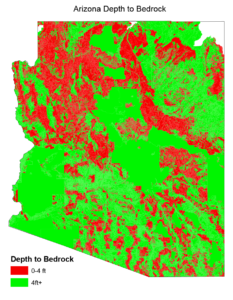
As noted previously, depth to bedrock is a critical indicator of the ease of cable installation, and the environmental impacts of the installation itself. Therefore, any soils with a bedrock layer at a starting depth shallower than 1.2 meters from the land surface were excluded as potential locations for undergrounding, as shown in the example in Figure A.

Figure 4 Depth to bedrock layer in Arizona

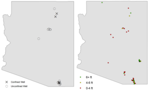
Shallow freshwater aquifers may present challenges for cable placement, and must be safeguarded carefully to avoid contamination or changes to water table hydraulic properties. Potential groundwater levels were surmised from data taken from government operated test wells located throughout the contiguous US. While the average depth of most aquifers is at least 11.6 meters from the surface in this dataset, depth levels have the potential to change within small geospatial areas and fluctuate with season. To obtain data on a manageable scale, depth-to-water in all government wells (2000 in total in the contiguous 48 states) was averaged and plotted. The structure of the aquifer (confined vs unconfined) was also collected for later usage during design phases. This as well as depth data must be further scrutinized as system design evolves. An example of both datasets is present in Figure C.

Figure 5 Groundwater conditions in Arizona

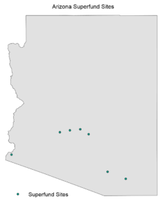
Existing Superfund and Brownfield sites were also tracked, regardless of contamination type, and should be avoided.

Figure 6 Superfund and Brownfield sites

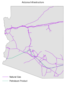
Finally, the location of manmade oil and gas infrastructure is displayed in Figure 7.

Figure 7 Oil and gas infrastructure in Arizona

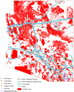
These layers were then combined to form a single “avoid undergrounding” layer (Figure 8), which will subsequently be combined with other soil characteristics to complete a final route map for the state of Arizona.

Figure 8 Final areas to avoid when undergrounding cables

 

“Amend Before Burial” Map Layer

 While some soil properties are difficult to correct, others may be readily altered to receive undergrounded cables without imposing unnecessary operational challenges. In other cases, no amendment/alteration is necessary at all, lowering costs and build time. For a soil to be considered amendable, it must not fall into the same area as a highlighted “avoid undergrounding” space when the two final maps are merged. For areas where this condition was met, we analyzed soil organic concentration[85], potential concrete corrosion capability[86], and soil order properties[87] to determine if the soil sample needs amendment. Amendment of soils usually occurs through usage of engineered silica fill to surround cables in trenches. Electrical and thermal properties of soils may also play a large role in the determination of potential amendments, yet due to their complexity, they are discussed elsewhere in this publication (in the section entitled Siting Based on Soil Resistivity Trends).

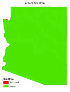
A comprehensive qualitative analysis of soil order properties can be found in the “Siting in the Context of Soil Mechanics” section. From this information, the extent of unsuitable soil types varied widely on a state-by-state basis. All soil orders previously deemed suitable were merged into a single green layer, erasing the colored distinction between orders.

 

Figure 9 Characterization of soil orders

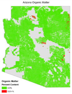
Furthermore, organic content plays an important role in the extent of heat dissipation for undergrounded cables. According to the literature, normal soils usually contain a composition of 5% organic matter.[88] Any soil that contains more organics than this baseline percentage is more likely to trap heat around operating cables. In this analysis, any soil samples containing more than 5% organics (Figure 10) were accordingly marked as requiring amendment before cable burial.

Figure 10 Organic matter content

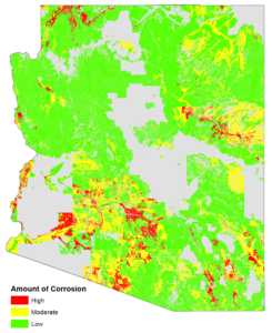
Qualitatively, we estimated concrete corrosion potential by combining the impact of salinity, acidity, sulfates, and other potentially harsh environmental components. Finally, we estimated corrosion potential, classifying areas either low, moderate, or high risk. Of these three distinctions, only areas which constituted a moderate or high risk were in need of amendment for the purposes of this analysis. Such areas are visualized in Figure 11.

Figure 11 Concrete corrosion potential

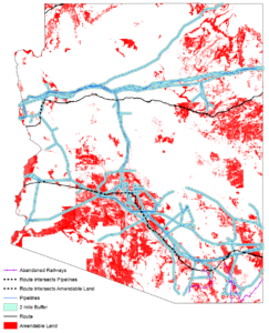
The final combination of these amend maps can be found in Figure 12. Pipeline infrastructure identical to that present in the final “avoid undergrounding” map was also represented at this stage, before the final combination of layers was executed.

Figure 12 Final areas in need of amendment when undergrounding cables

 

Final Cable Route

The combination of the “avoid” and “amend” map layers produced Figure 13. Although not explicitly shown, all information obtained from the previously described layers is contained in this figure. Areas that did not intersect any unfavorable avoid or amend conditions were assumed to be appropriate for underground burial without soil amendment. Nodal areas (which often center around large city centers) have the largest concentration of above ground cable configurations. Ultimately, 36% of mapped cable lines were placed above ground, with the remainder of lines remaining in an underground configuration. This percentage will most likely evolve as cable routes are mapped Eastward in the continental United States.

Figure 13 Final Western Pilot Project route

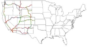
(Red line stretches denote above ground lines, blue line stretches denote underground lines requiring amendment before burial, and green line stretches denote underground lines requiring no amendment before burial.)[3]

 

Case Study 2 – Atlantic Coast Submarine Project

An offshore grid link may be a desirable method to connect the Northeastern and Southeastern coastal states. This feasibility study is a first investigation regarding this possibility and has considered biodiversity, chemo-physical, and anthropological concerns, which were classified as primary, secondary and supplemental concerns. Variables that were publicly available and considered relevant were gathered and overlapped using GIS tools. We present possible locations for the cable in three distinct scenarios.[4]

 

Chemo-physical Analysis

Chemo-physical analysis refers to data concerning the physical and chemical aspects of the offshore environment in the East Coast of the contiguous United States. To better understand this topic area, we studied sediment thickness, bathymetry, and seabed soil composition. Knowledge of sediment thickness was needed to identify sections of shallow soil that were inadequate for HVDC cable burial.[89] Although no mention was made within the metadata regarding the unit adopted in this dataset, it is reasonable to assume that “meters” was the intended unit. This dataset was compared to another showing the existence of communications cables in areas proximate to where HVDC cables might be buried, perhaps indicating the existence of appropriate conditions in the area.^[5]

Bathymetry is the depth, measured in meters, from the water surface to the seabed floor. Bathymetric differences can be represented graphically by isobath contours (lines which show the terrain present on the seabed) of equal relative depth.^[90] Data referring to bathymetry was collected from USGS in the form of two different GIS datasets.[91]˒[92] Both were combined to provide a high-resolution view of seabed depth. The isobaths contained in similar bathymetric intervals were colored with the same shade of green. As presented by an OSPAR Commission Report, “telecommunication cables installed over the last decade have been buried as [deep] as technically feasible, but not in areas with a water depth of more than 3,000 meters.”^[93] According to the same report, cables have already been placed in depths up to 1,000 and 1,200 meters.

Finally, the last dataset applied in this analysis was called “usSEABED facies data for the entire U.S. East Coast,” and was also collected from USGS datasets.[94] This data is a set of points for which a soil sample of known composition was collected; the data was first published in 2005, two years after data collection period occurred. This layer represented information such as the components and genesis of the seafloor, and was compiled from different sources that applied various methods in the collection. From the usSEABED dataset, points signaling the presence of carbon, volcanic rock, coral and/or another geochemical signal were highlighted, meaning some percentage of the component(s) was present in each sample (the presence of metamorphic rock and hard plant percentages were highlighted separately). While the conclusions drawn from this dataset are only approximations, such information may help to inform formal surveying efforts.[6]

 

Biodiversity Analysis

An additional aspect to consider when implementing a new electric grid is the impact it might have on localized biodiversity, particularly considering protected areas and habitats of marine species/coral. In order to predict and mitigate negative impacts associated with offshore HVDC cables, the following variables were included in the analysis: protected areas according to GAP statuses; Essential Fish Habitats (EFH) and Habitat Area(s) of Particular Concern (HAPC(s)), with data generated by the Florida Fish and Wildlife Conservation Commission (FWC), and the Fish and Wildlife Research Institute (FWRI) in association with the South Atlantic Fishery Management Council (SAFMC); Migratory Behavior – EFH Highly Migratory Species (HMS), with data generated by National Oceanic and Atmospheric Administration (NOAA); and Global Distribution of Coral Reefs, with data generated by the United Nations Environment Program’s World Conservation Monitoring Centre (UNEP-WCMC), the WorldFish Centre, World Resources Institute (WRI), and The Nature Conservancy (TNC).

As described in the WPP analysis, protected areas within the United States are classified in four categories (GAP Status 1 to 4) that are applicable in both marine and land environments. GAP Status 1 aquatic environments were avoided during the mapping process to maintain natural interaction between biotic and abiotic elements of these ecosystems. In addition to respecting designated GAP 1 lands, mapping of EFHs is also crucial to ensure that commercial fishing enterprises are protected during cable construction and operation. According to NOAA, EFHs are “those waters and substrate necessary to fish for spawning, breeding, feeding, or growth to maturity.”^[95] Among the EFHs, some are also classified as HAPC(s). This special category is considered a conservation priority, and is denoted as a “habitat type and/or geographic area identified by the eight regional fishery management councils and NOAA Fisheries as priorities for habitat conservation, management, and research.”^[96] A table of the species for which EFHs and/or HAPCs which were mapped is shown below in Table 1.[7]

Table 1 EFHs and HAPCs for prevalent species

Essential Fish Habitats	Habitat Areas of Particular Concern
Dolphin[97]	Dolphin[98]
Wahoo[99]	Wahoo[100]
Golden Crab[101]	Shrimp[102]
Shrimp[103]	Spiny Lobster[104]
Spiny Lobster[105]	Coastal Migratory Pelagics[106]
Coastal Migratory Pelagics[107]	Snapper Grouper[108]
Snapper Grouper[109]	Tilefish[8]

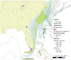
Figure 14 shows the areas where EFH, EFH-HAPC, and Coral Reefs were identified by the aforementioned sources (previously mentioned depth data is visualized in green contours on the same figure). The reef database plotted in orange was compiled by UNEP-WCM, the WorldFish Centre, WRI and TNC. It represents the global distribution of coral reefs (data collection was held from 1999 and 2002), with emphasis on warm-water coral reefs.^[9] Coral reefs in orange show that reefs in close proximity to the U.S. are concentrated in and around Florida’s South and Southeast Coast and near other islands South of the U.S.

Figure 14 Bathymetry, reefs, protected areas, and Essential Fish Habitats – North Carolina to Florida

As is true with coral reef locations, HAPCs are areas in which “the use of all bottom damaging gear is prohibited including bottom longline, trawl (bottom and mid-water), dredge, pot or trap, or the use of an anchor, anchor and chain, or grapple and chain by all fishing vessels.”^[110] Therefore, it is important to distinguish these areas from general HAPCs as well as Deepwater Coral HAPCs, which are a separate category defined after the establishment of HAPC areas. Scientific research points to the existence of high relief and hard bottom habitat areas that had not been included in the Coral HAPC boundaries. Figure 15 highlights both of these categories. It is crucial to note that various submarine cables intersect the three coral layers in the map.[111]˒[112]˒[113] This suggests that there is a method to burying submarine cables in Coral Habitat Areas. Nevertheless, guaranteeing the continuity of the natural lifecycle without great interferences will certainly require a deeper analysis by experts in localized marine biodiversity.

Figure 15 Coral EFH, EFH-HAEC and submarine cables

 

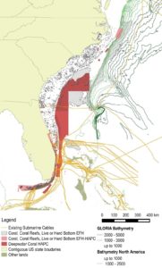
The habitat of some mammals was also considered as a variable to minimize the environmental impacts of an offshore HVDC cable.[114] Their distribution through the U.S. Atlantic Zone is presented below (Figure 16)[115]. All three layers cover the entire East Coast of the United States, which means that the cable will necessarily intercept those areas, if installed. This implies that the submarine cables presented in Figure 15 also cross those areas.

Figure 16 Marine mammals study areas and tracklines

 

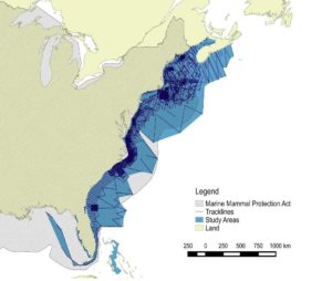
Similarly, we mapped animal migration, which highlighted the existent EFHs of Highly Migratory Species in the East Coast of the United States (according to data available from NOAA) previously. Most of these species are sharks^[10] and tunas^[11]; we included all other species in a third group termed “other species.”[12] All areas considered ideal for the cable burial, in terms of the chemo-physical conditions, are traversed by Highly Migratory Species EFH (especially by sharks[13]). Overlaying the Bathymetry and the information presented above, it was possible to clearly identify which species were present in the potential cable path.

The aforementioned shark population only circulate through the Gulf of Mexico or very close to the coast and in shallow waters. All other species inhabit or migrate through the area where the cable may be buried.[14] However, the circulation of those species throughout the entire East Coast of the United States did not impede the development of other offshore energy and infrastructure projects, positively impacting the feasibility assessment of this project. Nevertheless, the planning of any new marine infrastructure should still take place in a careful manner, considering the seasonal routes commonly traced by those species.

 

Anthropogenic Analysis

Aside from Biodiversity and Chemo-physical aspects, it is important to observe the anthropologic structures and activities that are present in the proposed placement area. To ensure that cables do not disrupt shipping channels, route planners must identify areas of high shipping traffic. While cables are usually buried at a safe depth in marine environments, seabed erosion and movements in the water can gradually expose the formerly buried cable. Human activity can further accelerate this process using anchors and because of trawling, processes that could expose cables and bring about life-threatening situations, for instance, a nautical vessel could capsize if its anchor were to catch on the exposed cable. In our attempts to identify risks for sea traffic, we considered several variables: shipping lanes[116], locations of ports, anchorage areas, and localized vessel density.

Shipping lanes are defined as routes regularly adopted by ships and are classified in the following seven categories:

1. Precautionary Areas, or those in which it is important to navigate with caution;
2. Speed Restriction Areas, or those in which the speed is seasonally reduced because of endangered species;
3. Particular Sensitive Areas, or those endangered by international maritime traffic;
4. Shipping Safety Fairways, or areas in which artificial structures are prohibited;
5. Areas to be Avoided, or areas that are hazardous for ships;
6. Recommended Routes, or those that should be chosen by ships for safety reasons; and
7. Traffic Separation Schemes/Traffic Lanes, where marine traffic is directed into designated routes.

Recommended Routes are only found close to Long Island, NY and along the coast of Maine. Speed Restriction Areas are the predominant shipping lane category used in the Eastern Atlantic. States in this category include: Georgia, South Carolina, North Carolina, Florida, New York, Virginia, Delaware, New Jersey, Connecticut, and Massachusetts. All shipping lanes should be avoided if possible.

Ports were georeferenced using newly created methodology, while similar information for deep-water ports (those located farther from the shoreline than traditional ports, which are used to load and unload large ships) was found in a premade public GIS dataset.[117]˒[118][119]All ports are spread in a non-equidistant manner along the East Coast, while deep-water ports can only be found off the coasts of California and Massachusetts. Consequently, deep-water ports should also be avoided by the cable burial path, which might be located a significant distance from the coastline. We recommend that conventional ports should be avoided by the offshore-onshore connections that will join the offshore cable with the underground grid in the continent, thus avoiding unnecessary disturbances to traffic during construction.

According to a NOAA description, “an anchorage area is a place where boats and ships can safely drop anchor.”[120] Such areas are created if required to improve safe and responsible navigation. Oftentimes there is high potential for ship crowding in areas specifically created for anchorages. Such areas should be avoided by any offshore grid cables and associated connections to prevent further overcrowding of such areas especially during the construction phase. Figure 17 represents the information described above, and proves that the areas and structures described above are very close to the coast, with the exception of the region between New Jersey and Massachusetts, where they might represent an obstacle for cable burial.

Figure 17 Shipping lanes, ports, and deepwater ports and anchorage sites

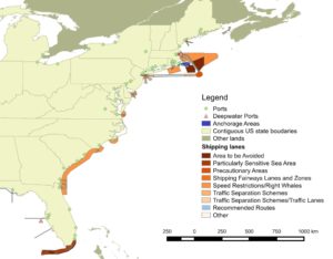
We also considered vessel density along the East Coast and mapped it separately from other concerns because of the difficulty of visualizing the associated data. This dataset in Figure 18 represents 2013 annual vessel traffic density for the contiguous United States offshore waters based on Automatic Identification System (AIS) monitoring.[121] This is a comprehensive density map that includes many types of vessels (cargo, fishing, passenger, etc.) and includes high to low density scaling that shows traffic concentration, not literal vessel counts. High vessel density is likely to occur around ports and narrow channels, based on data observation. Cable placement should purposely avoid high vessel density areas to prevent external vessel damage and ensure safe installation.

Figure 18 Vessel density for the year 2013

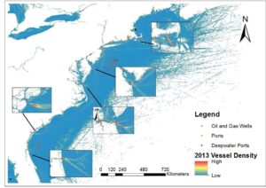
In addition to mapping of shipping-associated obstacles, we also considered marine based oil and gas infrastructure.[15] Data regarding petroleum product pipelines, product terminals, refineries, power plants, and points of underground storage were collected by U.S. Energy Information Administration (EIA)[122]. Coastal Energy Facilities (data collected from NOAA’s Bureau of Ocean Energy Management (BOEM)) and preexisting submarine cables were also accounted for in this sub-section. Figure 19 presents these components in the same map and were considered in the final suggested route for cable burial. The most obvious component of this figure is that cable intersections are common, implying that this is a possible configuration, given the cable function and operating party is known. We also considered fossil fuel well locations, power plant locations, and coastal energy facilities, particularly renewable-based facilities. Offshore wind planning zones and renewable energy leases, published by BOEM, were mapped[123]˒[124]; the leasing areas included the current leases and grants regarding renewable sources.[125] Finally, we analyzed disposal sites, military installations, unexploded ordinates[126] and wreckage sites[127] regarding the scenarios presented in the following section. Although these areas were not visualized in their own respective maps, it is important to state that many of them are already crossed by existing submarine cables, which decreases the relevance of those elements as a real concern for the cable burial.

Figure 19 Coastal energy facilities, oil and gas wells, pipelines, power plants, petroleum product terminals and petroleum refineries, and natural gas underground storage

 

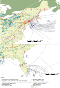
Offshore Grid Placement

Information pictured and/or described above was compiled into final maps displaying potential zones for cable placement. We classified chemo-physical, biodiversity, and anthropologic considerations into three categories: primary concerns, secondary concerns, and supplementary concerns (listed in Table 2 and visualized in Figure 20). Primary concerns are defined as factors that the cable placement must comply with without exception. Secondary concerns are factors that the cable placement should avoid if possible. Supplementary concerns are factors that the project developer can choose to adhere to (in order to lower risk) or ignore for the sake of cost. Subsequently, these scenarios were built based on these classifications. The final decision on the cable placement will likely be a compromise between results from this feasibility analysis, a financial evaluation, and a developer-driven analysis. The classification of primary, secondary, and supplemental concerns may evolve over time with more detailed feasibility and design efforts.

Table 2 Primary, secondary, and supplemental concerns for cable placement

Primary Concerns
Bathymetry	Optimal water depth to place is between 1000~3000 meters
Sediment thickness	Optimal seabed depth to bury is at least 1m.
Deepwater ports	Must avoid existing structures.
Military installations	Must avoid existing structures.
Oil and gas wells	Must avoid existing structures.
Coastal energy facilities	Must avoid existing structures.
GAP status 1	Permanent protection from land cover conversion.
Secondary Concerns
Seabed Type	Avoid hard seabed bottom if possible
Vessel density	Avoid high vessel density area if possible.
Wind planning zone	Avoid planning zone if possible.
Renewable energy lease	Avoid lease zone if possible.
Coral	Avoid deep-water HAPC Coral zone if possible.
Supplementary Concerns
Expanded coral	Choose to avoid coral EFH and EFH HAPC.
Anchorage Area	Choose to avoid anchorage area.
Disposal Sites	Choose to avoid disposal sites.
Unexploded ordnance	Choose to avoid unexploded ordnance.

 

Figure 20 Primary, secondary, and supplementary concerns visualized together

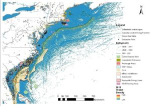
Having set out the possible cable routes, we also needed to demonstrate the feasibility of building connections between the offshore cable and the onshore underground grid. In assessing the environmental conditions, we avoided military installations, coastal energy facilities, oil and gas wells, ports and deep-water ports, high vessel density, as well as GAP status 1 protected areas. We considered areas with suitable soils and at least a 1.2 meter depth to the bedrock most favorable for offshore-onshore connections. Based on that, we have suggested three potential locations for onshore-offshore connection points in Delaware, New Jersey, and Georgia.

 

Conclusion

This section aimed to give concreteness to the ambitious vision of the creation of a HVDC underground network in the contiguous United States. By collecting publicly available data and analyzing the distribution of those variables in a geo-referred manner, this study was able to pinpoint what seems to be an optimistic scenario for the construction of an HVDC cable network with both onshore and offshore components. Considering the way existing cables interact with relevant variables, it seems to be quite feasible to build the system without causing serious and long-lasting impacts on the surrounding environment, humans, or wildlife.

 

Notes

[1] HVDC cables will only generate static magnetic fields; therefore, induction does not impact calculations for the general design analysis.

[2] The air quality model described is proprietary, and therefore not described in its entirety. All results are simulated estimations and should be taken as a finite descriptor of system effects; further refinement may be required before results can be considered in design and system planning. Please contact authors if you would like to request more information about the source data used or calculation steps.

[3] This representation of the Western Pilot project should not be regarded as a final design for the system, it is subject to change and evolve as data is further collected and analyzed.

[4] This case study is meant to provide an extremely comprehensive view of the potential issues that may be associated with cable placement, using public data outlets as the main information source. Actual construction plans may necessitate the gathering of additional data or disregard certain datasets mentioned in this work.

[5] This dataset will be presented later in this report. Although, other reliable sources must be consulted before the installation of the offshore cable.

[6]  The sediment thickness and bathymetric information presented appear to be accurate and consistent. The information regarding soil composition, however, should be further verified applying other sources such as private firms, scholars, or government agencies who have worked directly in these offshore areas. Despite the broad visualization of soil composition this USGS dataset has enabled, the data collection dates do vary from 1840 to 2003, meaning that there is the possibility that some of the information has significantly changed. In addition, the absence of data from some of the points does not necessarily imply the absence of a mineral/organic soil component in the sample (this can occur due to unavailable data), which could also undermine conclusive statements regarding soil composition.

[7] A Snapper Grouper EFH layer could not be visualized and is not included in the corresponding map.

[8] Website currently under construction, originally used metadata not available. Original link to data available upon request.

[9] “Approximately 85% of this dataset originates from the Millennium Coral Reef Mapping Project, of which 35% was validated (by IMaRS-USF and IRD-Noumea) and 50% remains unvalidated (but was interpreted by UNEP-WCMC). Millennium Coral Reef Mapping Project products (validated or not) are at a consistent 30 m resolution.” (Quotes contained in the “Global Distribution of Coral Reefs (2010)” GIS data documentation).

[10] The species of sharks included in this report are those available in NOAA GIS dataset on Highly Migratory Species: Caribbean Reef Shark, Common Thresher Shark, Dusky Shark, Finetooth Shark, Great Hammerhead Shark, Lemon Shark, Longfin Mako Shark, Oceanic Whitetip Shark, Night Shark, Nurse Shark, Porbeagle Shark, Sandbar Shark, Sand Tiger Shark, Scalloped Hammerhead Shark, Shortfin Mako Shark, Silky Shark, Spin Shark, Tiger Shark, Whale Shark, White Shark, Atlantic Sharpnose Shark, Bigeye Thresher Shark, Basking Shark, Bignose Shark, Blacknose Shark, Blacktip Shark, Angel Shark, Blue Shark, Bull Shark and Bonnethead Shark.

[11] The species of tuna included in this report are those available in NOAA GIS dataset on Highly Migratory Species: Skipjack Tuna, Yellowfin Tuna, Bluefin Tuna, Albacore Tuna and Bigeye Tuna.

[12] “Other species” include: Longbill Spearfish, White Marlin, Sailfish, Swordfish and Blue Marlin.

[13] Few species of sharks have essential habitats outside of the desired bathymetric clarification: Caribbean Reef Shark, Finetooth Shark, Lemon Shark, Nurse Shark, Whale Shark, Sandbar Shark, Spinner Shark, White Shark, Atlantic Sharpnose Shark, Blacknose Shark, Blacktip Shark, Bull Shark, and Bonnethread Shark.

[14] A complete set of maps for each of the affected species available upon request.

[15] Utilized data was published in 2015, with collection occurring from 1975 to 1984.

 

Citations

[1] Ophardt, Charles E. “What are Physical Properties and Changes?” Virtual Chembook: Elmhurst College. Last modified 2003. http://chemistry.elmhurst.edu/vchembook/104Aphysprop.html

[2] Ibid. YourDictionary. “Examples of Physical Properties.” Last modified 2017. http://examples.yourdictionary.com/examples-of-physical-properties.html.

[3] ” Ibid. Keener-Chavis, Paula and Leslie Reynolds Sautter. “Chapter II: Physical and Chemical Properties of the Ocean.” Of Sand and Sea: Teaching From the Southeastern Shorline (Charleston, SC: S.C. Sea Grant Consortium, August 2002), 19-23.

[4] Plant and Soil Sciences ELibrary. “Soil Genesis and Development, Lesson 5 – Soil Classification and Geography.” Last modified 2017. http://passel.unl.edu/pages/informationmodule.php?idinformationmodule=1130447032.

[5] National Resources Conservation Service Soils: United States Department of Agriculture. “The Twelve Orders of Soil Taxonomy.” https://www.nrcs.usda.gov/wps/portal/nrcs/detail/soils/edu/?cid=nrcs142p2_053588.

[6] “Soil Genesis and Development.” University of Florida Soil and Water Science. “Soil Orders.” Last modified 2017. http://ufgrunwald.com/soil-orders/.

[7] “Soil Genesis and Development.”

[8] Ibid. McDaniel, Paul. “The Twelve Soil Orders.” The Twelve Soil Orders: Soil Taxonomy. http://www.cals.uidaho.edu/soilorders/orders.htm.

[9] “Soil Genesis and Development.”

[10] McDaniel. “The Twelve Soil Orders.”

[11] “Soil Genesis and Development.”

[12]. “Soil Orders.” McDaniel. “The Twelve Soil Orders.”

[13] Ibid.

[14] “Soil Genesis and Development.” McDaniel. “The Twelve Soil Orders.”

[15] “Soil Orders.” Lindbo, Dave. “Soil Types.” Soil Science Society of America. Last modified 2017. https://www.soils.org/discover-soils/soil-basics/soil-types.

[16] “Soil Genesis and Development.” “Soil Orders.” WindWolf. “Feet on the Ground…Soil: The Ultisols.” Last modified November 16, 2016. http://sci.windwolf.org/soil/orders11.htm. Lindbo. “Soil Types.”

[17] “Soil Genesis and Development.”  Lindbo. “Soil Types.”

[18] Beaty, H. Wayne and Donald G. Fink, ed. Standard Handbook for Electrical Engineers, 16^th ed. New York: McGraw Hill, 2013.

[19] Ibid

[20] Parmar, Deepak and Jan Steinmanis. “Underground Cables Need a Proper Burial.” T&D World Magazine, April 1, 2003. http://www.tdworld.com/underground-tampd/underground-cables-need-proper-burial.

[21] Molburg, J.C., J.A. Kavicky, and K.C. Picel. The Design, Construction, and Operation of Long-Distance High-Voltage Electricity Transmission Technologies. Lemont, IL: Argonne National Laboratory, November 2007.

[22] Pavement Interactive. “HMA Pavement.” Last modified 2012. http://www.pavementinteractive.org/article/hma-pavement/.

[23] GlobalSecurity.org. “Chapter 5 – Subgrades and Base Courses.” Last modified 2017. http://www.globalsecurity.org/military/library/policy/army/fm/5-430-00-1/CH5.htm.

[24] AFS and the Institute. “Bases and Subbases.” http://www.afsinc.org/content.cfm?ItemNumber=7098.

[25] Mitigating the Impacts of Electric Transmission Lines. PPT. Sacramento: California Institute for Energy and Environment. November 2012.

[26] Railwaysubstructure.org. “Basic Track Components.” http://railwaysubstructure.org/railwiki/images/2/29/Basic_Track_Components.png.

[27] The Engineering Toolbox. “Thermal Resistivity and Conductivity.” http://www.engineeringtoolbox.com/thermal-resistivity-d_1053.html.

[28] E&S Grounding Solutions. “What Is Soil Resistivity Testing?” Last modified 2015. http://www.esgroundingsolutions.com/what-is-soil-resistivity-testing/.

[29] Lasance, Clemens. “How Thermal Conductivity Relates to Electrical Conductivity.” Electronics Cooling, May 1, 2000. https://www.electronics-cooling.com/2000/05/how-thermal-conductivity-relates-to-electrical-conductivity/.

[30] Ibid.

[31] Tuller, Markus and Dani Or. “Soil Temperature and Heat Flow.” University of Connecticut Lecture Material for CE/ENVE 320-Vadose Sone Hydrology/ Soiul Physics Spring 2004. http://studylib.net/doc/8839561/soil-temperature-and-heat-flow.

[32] Switzer, Keith. “Achieving an Acceptable Ground in Poor Soil.” EC&M, October 1, 1998. http://ecmweb.com/content/achieving-acceptable-ground-poor-soil.

[33] Ibid.

[34] Why Measure Soil Resistivity? Dover, NH: AEMC Instruments, August 2002. http://www.transcat.com/media/pdf/App-Ground-SoilResistivity.pdf.

[35] Earth Ground Resistance – Principals, Testing Methods, and Applications. Everett, WA: Fluke Corporation. http://support.fluke.com/find-sales/Download/Asset/2633834_6115_ENG_A_W.PDF .

[36] Switzer. “Achieving an Acceptable.”

[37] Ibid.

[38] Why Measure Soil Resistivity?

[39] “Classifying Electrolytes.” https://www.stolaf.edu/depts/chemistry/courses/toolkits/121/js/naming/elec.htm.

[40] Chieh, Chung. “Electrolytes.” University of Waterloo – Science. http://www.science.uwaterloo.ca/~cchieh/cact/c120/electrolyte.html.

[41] Helmstine, Anne. “Electrolytes  – Strong, Weak, and Non Electrolytes.” Science Notes, April 30, 2014. Last modified September 24, 2017. https://sciencenotes.org/electrolytes-strong-weak-and-non-electrolytes/.

[42] He, Jinliang, Rong Zeng, and Bo Zhang. Methodology and Technology for Power System Grounding. Singapore: John Wiley & Sons Singapore Pte. Ltd. 2013.

[43] Campbell, Gaylon S., and Keith L. Bristow. The Effect of Soil Thermal Resistivity (RHO) an Underground Power Cable Installations. Pullman, WA: Thermal Decagon Devices, Inc., 2014.

[44] Why Measure Soil Resistivity? Dover, NH: AEMC Instruments, August 2002. http://www.transcat.com/media/pdf/App-Ground-SoilResistivity.pdf.

[45] Durgin, Philip B. and Thomas M. Young, ed. STP 1161: Leak Detection for Underground Storage Tanks. Philadelphia, PA: ASTM, 1993.

[46] Bailey, William H., Deborah E. Weil, and James R. Stewart. HVDC Power Transmission Environmental Issues Review. Oak Ridge, TN: Oak Ridge National Laboratory, April 1997.

[47] UCSG. “A summary of the relationship between GAP Status Codes and IUCN Definitions.” National GAP Analysis Program – Core Science Analytics and Synthesis. Last modified September 13, 2012.  http://gapanalysis.usgs.gov/blog/iucn-definitions/.

[48] Ibid.

[49] U.S. Geological Survey. published 5/5/2016. Native American Reservations. Protected Areas Database v1.4.

[50] Assessing and Managing the Ecological Impacts of Paved Roads. Washington, D.C.: National Academy of Sciences, 2005. 63-64.

[51] Rosenberg, Henrik. Electric Power, HVDC from Land to Off-shore Structures Utilizing Sea-electrodes for Return Current, Concerns and Precautions with Regard to Environment and Corrosion. Denmark: Balslev Consulting Engineers. The Essential Chemical Industry. “Chlorine.” Last modified 2016. http://www.essentialchemicalindustry.org/chemicals/chlorine.html.

[52] Ibid.

[53] Center for Disease Control and Prevention. “CHLORINE: Damaging Agent.” The National Institute for Occupational Safety and Health (NIOSH). Last modified May 26, 2015. http://www.cdc.gov/niosh/ershdb/emergencyresponsecard_29750024.html.

[54] Andrulewicz, Eugeniusz, Dorota Napierska, and Zbigniew Otremba. “The Environmental Effects of the Installation and Functioning of the Submarine SwePol Link HVDC Transmission Line: A Case Study of the Polish Marine Area of the Baltic Sea.” Journal of Sea Research 49, no. 4 (2003). doi:10.1016/s1385-1101(03)00020-0.

[55] Ibid.

[56] Ibid.

[57] Ardelean, Mircea and Philip Minnebo. JRC Technical Reports: HVDC Submarine Power Cables in the World. Brussels, Belgium: European Joint Research Commission, 2015.

[58] National Ocean Service: National Oceanic and Atmospheric Administration U.S. Department of Commerce. “How far does light travel in the ocean?” Ocean Facts. https://oceanservice.noaa.gov/facts/light_travel.html.

[59] Ardelean and Minnebo. JRD Technical Reports.

[60] Ibid

[61] Bailey, Weil, and Stewart. HVDC Power Transmission.

[62] Ibid

[63] J. Droppo, J. G.”Field Determinations of HVDC Ozone Production Rates.” IEEE Transactions on Power Apparatus and Systems PAS-100, no. 2 (1981). doi:10.1109/tpas.1981.316962.

[64] Bailey, Weil, and Stewart. HVDC Power Transmission.

[65] Ibid

[66] Green Facts. “1. What are static electric and magnetic fields?” Static Fields. Last modified 2017. http://www.osti.gov/servlets/purl/580576-BUAbF9/webviewable/.

[67] Schmidt, G., B. Fiegl, and S. Kolbeck. “HVDC Transmission and the Environment.” Power Engineering Journal 10, no. 5 (1996). doi:10.1049/pe:19960503.

[68] Supe, A. and J. Porins. “Interaction Between Electromagnetic Field and Optical Signal Transmission in Fiber Optics.” Electronics and Electrical Engineering 122, no. 6 (2012), 83–86.

[69]  Technical Guidelines: Pathway Separation Between Telecommunication Cables and Power Cables. Atlanta, GA: Superior Essex, November 7, 2016.

[70] Lilliestierna, Andreas, and Johan Utas. “Thermal Classification of Cable Route.” Master’s thesis, Chalmers University of Technology, 2015. http://publications.lib.chalmers.se/records/fulltext/223457/223457.pdf.

[71] New England Clean Power Link HVDC Transmission Project Presidential Permit Application. Champlain, VT: May 2014.

[72] Bailey, Weil, and Stewart. HVDC Power Transmission.

[73] Ibid

[74] Ibid

[75] Ibid

[76] United States Environmental Protection Agency. “NAAQS Table.” Last modified December 20, 2016. https://www.epa.gov/criteria-air-pollutants/naaqs-table.

[77] Ozone Services and OzoneLab, “Ozone Levels and Their Effects.” Ozone in the Air. http://www.ozoneservices.com/articles/007.htm.

[78] U.S. Geological Survey, 2006. Minimum Depth-to-Bedrock values provided by USDA/NRCS’s STATSGO2.

[79] U.S. Census Bureau, DOD, DHS, 2016. TIGER/Line Shapefile, 2016. U.S., Military Installation National Shapefile.

[80] U.S. Geological Survey. Protected Areas Database of the United States (PAD-US)

[81] U.S. Energy Information Agency, 2016. Oil and Gas Infrastructure (sub-sets analyzed include: HGL Pipelines, Natural Gas Interstate and Intrastate Pipelines, Natural Gas Underground Storage Facilities, Petroleum Product Pipelines, Petroleum Product Terminals, Petroleum Refineries, Power Plants, Crude Oil Pipelines, Tight Oil Shale Gas Plays).

[82] U.S. Energy Information Agency, U.S. Department of Labor, Mine Safety and Health Administration, 2014. Coal Mines, Surface and Underground.

[83] Environmental Protection Agency, Geospatial Data Download Service (2017). https://www.epa.gov/enviro/geospatial-data-download-service.

[84] U.S. Geologic Survey, Advisory Committee on Water Information. Welcome to the National Ground-Water. https://cida.usgs.gov/ngwmn/index.jsp.

[85] USDA Natural Resources Conservation Service, 2017. Web Soil Survey: Organic Matter Concentration.

[86] USDA Natural Resources Conservation Service, 2017. Web Soil Survey: Concrete Corrosion Potential.

[87] Paul Reich, USDA-NRCS & FAO-UNESCO, last modified: 2005. Global Soil Regions [GIS].

[88] Ionita, I., et al. “The Behavior of Underground Power Cables Under the Action of Stress Factors.” Romanian Journal of Physics 59, no. 9-10 (2014).

[89] NOAA, National Centers for Environmental Information, NESDIS, U.S. Department of Commerce, 2013. Total Sediment Thickness of the World’s Oceans & Marginal Seas, version 2.

[90] U.S. Geological Survey, Government of Canada. Natural Resources Canada. Canada Centre for Remote Sensing. The Atlas of Canada e Instituto Nacional de Estadistica Geografia e Informatica, 2004. Census USGS Small-scale Dataset – North American Atlas – Bathymetry 200406 Shapefile. http://dds.cr.usgs.gov/pub/data/nationalatlas/bathy0m_shp_nt00296.tar.gz.

[91] U.S. Geological Survey, Government of Canada, Natural Resources Canada, Canada Centre for Remote Sensing, The Atlas of Canada e Instituto Nacional de Estadistica Geografia e Informatica, 2004. Census USGS Small-scale Dataset – North American Atlas – Bathymetry 200406 Shapefile.

[92] U.S. Geological Survey, EEZ-Scan 87 Scientific Staff, 1991. U.S. Atlantic East Coast bathymetry contours (EGLORIA_CNT).

[93] Merck, Thomas and Ralf Wasserthal. Assessment of the environmental impacts of cables. London, UK: OSPAR Commission Biodiversity Series, 2009.

[94] U.S. Geological Survey, University of Colorado, 2005. ATL_FAC: usSEABED facies data for the entire U.S. Atlantic Coast, 1840-2003.

[95] Essential Fish Habitat Consultation Guidance. Silver Spring, MD: National Marine Fisheries Service Office of Habitat Conservation, 2004. 3.

[96] Regional Use of the Habitat Area of Particular Concern (HAPC) Designation. Dover, DE: Mid-Atlantic Fishery Management Council, September 22, 2016. 1.

[97] Florida Fish and Wildlife Conservation Commission-Fish and Wildlife Research Institute, 2005. Dolphin and Wahoo EFH-HAPC.

[98] Ibid

[99] Ibid

[100] Ibid

[101] Florida Fish and Wildlife Conservation Commission-Fish and Wildlife Research Institute, 2008. Golden Crab Essential Fish Habitats.

[102] Florida Fish and Wildlife Conservation Commission-Fish and Wildlife Research Institute, 2005. Shrimp RFH-HAPC.

[103] Florida Fish and Wildlife Conservation Commission-Fish and Wildlife Research Institute, 2008. Shrimp Essential Fish Habitat.

[104] Florida Fish and Wildlife Conservation Commission-Fish and Wildlife Research Institute, 2005. Spiny Lobster EFH-HAPC.

[105] Florida Fish and Wildlife Conservation Commission-Fish and Wildlife Research Institute, 2008. Spiny Lobster Essential Fish Habitat.

[106] Florida Fish and Wildlife Conservation Commission (FWC), Fish and Wildlife Research Institute (FWRI), South Atlantic Fishery Management Council (SAFMC), 2005.  Coastal Migratory Pelagics Essential Fish Habitat – Habitat Area of Particular Concern (EFH-HAPC).

[107] Florida Fish and Wildlife Conservation Commission (FWC), Fish and Wildlife Research Institute (FWRI), South Atlantic Fishery Management Council (SAFMC), 2005.  Coastal Migratory Pelagics EFH.

[108] Florida Fish and Wildlife Conservation Commission-Fish and Wildlife Research Institute, 2005. Snapper Grouper EFH-HAPC.

[109] Florida Fish and Wildlife Conservation Commission-Fish and Wildlife Research Institute, 2015. Snapper Grouper Essential Fish Habitat.

[110] Florida Fish and Wildlife Conservation Commission-Fish and Wildlife Research Institute. ”Deep Water Coral HAPCs.” Last modified January 14, 2016.

[111] NOAA, DOC, NOS, OCM, 2016. NOAA Charted Submarine Cables in the United States as of December 2012.

[112] Florida Fish and Wildlife Conservation Commission (FWC), Fish and Wildlife Research Institute (FWRI), 2015. Deepwater Coral HAPCs.

[113] Florida Fish and Wildlife Conservation Commission-Fish and Wildlife Research Institute Florida Fish and Wildlife Conservation Commission (FWC), Fish and Wildlife Research Institute (FWRI), Coastal and Marine Resources Assessment (CAMRA), 2005. Coral, Coral Reef and Live Hard Bottom EFH-HAPC.

[114] Department of Commerce (DOC), National Oceanic and Atmospheric Administration (NOAA), National Ocean Service (NOS) 2016. Marine Mammal Protection Act.

[115] BOEM, 2012. Wildlife Survey Tracklines, ATL_WILDLIFE_SURVEYS.

[116] Department of Commerce (DOC), National Oceanic and Atmospheric Administration (NOAA), National Ocean Service (NOS), Office of Coast Survey (OCS). “FGDC Content Standard for Digital Geospatial Metadata.” Last modified 2015.

[117] DOC, NOAA, NOS, OCM, 2015. Deepwater Ports in US waters.

[118] NOAA, 2015. Deepwater Ports in US Waters as of August 2013.

[119] Maritime Administration, U.S. Department of Transportation, 2015. Vessel Calls in U.S. Ports, Selected Terminals and Lightering Areas: Privately-owned, oceangoing merchant vessels over 1,000 gross tons.

[120] NOAA Office for Coastal Management. “Anchorage Areas.” Last modified 2015.

[121] NOAA Office for Coastal Management. FGDC Content Standard for Digital Geospatial Metadata. Charleston, SC: NOAA, 2015.

[122] U.S. Energy Information Agency, 2016. Oil and Gas Infrastructure

[123] BOEM, 2016. BOEM Lease Areas Shapefile.

[124] BOEM, Wind Planning Areas Shapefile.

[125] BOEM Lease Areas Shapefile. Sterling, VA: Bureau of Ocean Energy Management, December 15, 2016.

[126] DOC, NOAA, NOS, 2009. Unexploded Ordinances in US waters as of February 2014.

[127] DOC, NOAA, NOS, Hydrographic Surveys Division (HSD), 2009. Office of Coast Survey’s Automated Wreck and Obstruction Information System.